|
A New View of Statistics | |
 Let's
use the same example that I used to introduce the concept of statistical
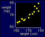
models. As you can see, data for two variables like weight and height scream
out to have a straight line drawn through them. The straight line will allow us
to predict any person's weight from a knowledge of that person's height. Obviously,
the prediction won't be perfect, so we will also be able to say how strong the
linear relationship is between weight and height, or how well the straight line
fits the data (the goodness of fit).
Here's how we represent the model:
model: numeric <= numeric
example: weight <= height
You normally think about a straight line as Y = mX + c, where m is the slope
and c is the intercept. The way I would write this relationship, using the above
notation, is simply Y <= X. We don't have to worry about showing
the constants, but the stats program worries about them. They're the parameters
in the model.
The Slope
The most interesting parameter in a linear
model is usually the slope. If the slope is zero, the line is flat, so there's
no relationship between the variables. In the example, the slope is about 0.75
kg per cm (an increase in weight of 0.75 kg for each cm increase in height).
We can also calculate the slope in two ways that don't have those ugly units
(kg per cm).
One way is to calculate the percent change in weight per percent change in height. It's unusual, but sometimes it's the best way, especially for variables that need log transformation. The slope expressed as % per % comes directly out of the analysis of log-transformed variables.
The other way to remove the units is to normalize the two variables
by dividing their values by their standard deviations, then fit the straight
line. The resulting slope is known as a standardized regression coefficient.
It represents the change in weight, expressed as a fraction of the standard
deviation, per standard deviation change in height. You can also generate it
by multiplying the slope (in kg per cm) by the ratio of the standard deviations
for height over the standard deviation for weight. In a simple linear regression,
the value of the standardized regression coefficient is exactly the same as
the correlation coefficient, and you can interpret its magnitude in the same
way. In the example, the value is about 0.9, or a difference of 0.9 standard
deviations in weight per change of one standard deviation in height. That's
a really strong relationship!
Goodness of Fit
The stats program works out values for the
slope and intercept (the parameters) that give the best fit. I'll explain how
after I've dealt with all four simple models. Meanwhile, we want a measure of
how good the fit is. The correlation coefficient is
one such measure. Another way to represent the fit is to square the correlation
coefficient, multiply it by 100, then call the result the percent of variance
explained, or percent R2. For example,
the R2 represents the proportion of variation
in weight that can be attributed to height, when there is a linear relationship
between weight and height. A correlation of 0.9 is equivalent to an R2
of 0.81 or 81%. I'll explain more about goodness
of fit in a few pages' time.
The p value or the confidence interval for the correlation coefficient tell us how good the fit is likely to be in the population. The program can also give confidence intervals or p values for the slope and intercept. The correlation coefficient can be considered as a test statistic for whether the line fits the data at all. But stats programs can also produce another statistic for this purpose, called the F ratio. The values for F are quite different from those for r, but there is a one-to-one relationship between them, and the r and the F have the same p value for a given sample.