Making Meaningful Inferences About Magnitudes Alan M Batterham, Will G Hopkins Sportscience 9, 6-13, 2005 (sportsci.org/jour/05/ambwgh.htm)
|
|
Update 2013: See this In-brief item for a more succinct slideshow about inference and a comprehensive treatment of effect magnitudes. Update 2009: Minor updates to the slideshow for consistency with a more recent article (Hopkins, 2007) explaining mechanistic vs clinical/practical inferences. Other Approaches to Inferences Appendix: Examples of Reporting
of Magnitude-Based Inferences Researchers usually conduct a study by selecting a sample of subjects from some population, collecting the data, then calculating the value of a statistic that summarizes the outcome. In almost every imaginable study, a different sample would produce a different value for the outcome statistic, and of course none would be the value the researchers are most interested in–the value obtained by studying the entire population. Researchers are therefore expected to make an inference about the population value of the statistic when they report their findings in a scientific journal. In this article we first critique the traditional approach to inferential statistics, the null-hypothesis test. Next we explain confidence limits, which have begun to appear in publications in response to a growing awareness that the null-hypothesis test fails to deal with the real-world significance of an outcome. We then show that confidence limits alone also fail, before outlining our own approach and other approaches to making inferences based on meaningful magnitudes. The
Null-Hypothesis Test
The almost universal approach to inferential statistics has been the null hypothesis test, in which the researcher uses a statistical package to produce a p value for an outcome statistic. The p value is the probability of obtaining any value larger than the observed effect (regardless of sign), if the null hypothesis were true. When p<0.05 the null hypothesis is rejected and the outcome is said to be statistically significant. In an effort to bring meaning to this deeply mysterious approach, many researchers misinterpret the p value as the probability that the null hypothesis is true, and they misinterpret their outcomes accordingly. Jacob Cohen, in his classic article "The Earth is Round (p<0.05)", summed up this confusion by concluding that significance testing “does not tell us what we want to know, and we so much want to know what we want to know that, out of desperation, we nevertheless believe that it does!” (Cohen, 1994, p.997) Readers may also wonder what is sacred about p<0.05? The answer is nothing. Ronald Fisher, the statistician and geneticist who championed the p value, correctly asserted that it was a measure of strength of evidence against the null hypothesis, and that "we shall not often go astray if we draw a conventional line at 0.05" (Fisher, 1950). It was not Fisher’s intention that p<0.05 should be used as an absolute decision rule. Indeed, he would almost certainly have endorsed the suggestion of Rosnow and Rosenthal (1989) that “surely God loves the 0.06 nearly as much as 0.05” (p.1277). Regardless of how the p value is interpreted, hypothesis testing is illogical, because the null hypothesis of no relationship or no difference is always false–there are no truly zero effects in nature. Indeed, in arriving at a problem statement and research question, researchers usually have good reasons to believe that effects will be different from zero. The more relevant issue is not whether there is an effect, but how big it is. Unfortunately, the p value alone provides us with no information about the direction or size of the effect or, given sampling variability, the range of feasible values. Depending, inter alia, on sample size and variability, an outcome statistic with p<0.05 could represent an effect that is clinically, practically, or mechanistically irrelevant. Conversely, a non-significant result (p>0.05) does not necessarily imply that there is no worthwhile effect, as a combination of small sample size and large measurement variability may mask important effects. An over-reliance on p values may therefore lead to unethical errors of interpretation. As Rozeboom (1997) stated, “Null-hypothesis significance testing is surely the most bone-headedly misguided procedure ever institutionalized in the rote training of science students” (p.35). Confidence
Intervals
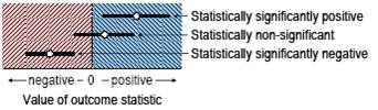
In response to these and other critiques of hypothesis testing, confidence intervals are beginning to appear in research reports. The strict definition of the confidence interval is hotly debated, but most if not all statisticians would agree that the confidence interval is the range within which we would expect the value of the statistic to fall, if we were to repeat the study with a very large sample. More simply, it is the likely range of the true, real, or population value of the statistic. For example, consider a two-group comparison of means, in which we observe a mean difference of 10 units, with a 95% confidence interval of 6 to 14 units (or lower and upper confidence limits of 6 and 14 units). In plain language, we can say that "the true difference between groups could be somewhere between 6 and 14 units", where could refers to the probability used for the confidence interval. A confidence interval alone or in conjunction with a p value still does not overtly address the question of the clinical, practical, or mechanistic importance of an outcome. Given the meaning of the confidence interval, an intuitively obvious way of dealing with magnitude of an outcome statistic is to inspect the magnitudes covered by the confidence interval and thereby make a statement about how big or small the true value could be. The simplest scale of magnitudes we could use has two values: positive and negative for statistics like a correlation coefficients, differences in means and differences in frequencies, or greater than unity and less than unity for ratio statistics like relative risks. If we apply the confidence interval for an outcome statistic to such a two-level scale of magnitudes, we can make one of three inferences: the statistic could only be positive, the statistic could only be negative, or the statistic could be positive and negative. The first two inferences are equivalent to the value of the statistic being statistically significantly positive and statistically significantly negative respectively, whereas the third is equivalent to the value of the statistic being statistically non-significant. We illustrate these three inferences in Figure 1.
This equivalence of confidence intervals and statistical significance is a well-known corollary of statistical first principles, and we will not explain it further here. But we stress that confidence intervals do not represent an advance on null hypothesis testing, if they are interpreted only in relation to positive and negative values or, equivalently, the zero or null value. Magnitude-Based
Inferences
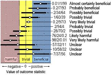
The problem with a two-level scale of magnitude is that some positive and negative values are too small to be important in a clinical, practical or mechanistic sense. The simplest solution to this problem is use a three-level scale of magnitude: substantially positive, trivial, and substantially negative, defined by the smallest important positive and negative values of the statistic. In Figure 2 we illustrate a crude approach to the various magnitude-based inferences for a statistic with substantial values that are clinically beneficial or harmful.
There is no argument about the inferences shown in Figure 2 for confidence intervals that lie entirely within one of the three levels of magnitude (harmful, trivial, beneficial). For example, the outcome is clearly harmful if the confidence interval is entirely within the harmful range, because the true value could only be harmful (where could only be refers to a probability somewhat more than the probability level of the confidence interval). A confidence interval that spans all three levels is also relatively easy to deal with: the true value could be harmful and beneficial, so the outcome is unclear, and we would need to do more research with a larger sample or with better measures to resolve the uncertainty. But how do we deal with a confidence interval that spans two levels–harmful and trivial, or trivial and beneficial? In such cases the true value could be harmful and trivial but not beneficial, or it could be trivial and beneficial but not harmful. Situations like these are bound to arise, because a true value is sometimes close to the smallest important value, and even a narrow confidence interval will sometimes overlap trivial and important values. It would therefore be a mistake to conclude that the outcome was unclear. For example, a confidence interval that spans beneficial and trivial values is clear in the sense that the true value could not be harmful. One option for dealing with a confidence interval that spans two regions is to make the inference not harmful, but the reader will then be in doubt as to which of the other two outcomes (trivial or beneficial) is more likely. A preferable alternative is to declare the outcome as having the magnitude of the observed effect, because in almost all studies the true value will be more likely to have this magnitude than either of the other two magnitudes. Furthermore, there is an understandable tendency for researchers to interpret the observed value as if it were the true value. We regard the approach summarized in Figure 2 as crude, because it does not distinguish between outcomes with confidence intervals that span a single magnitude level and those that start to overlap into another level. Furthermore, the researcher can make incorrect inferences comparable to the Type I and Type II errors of null-hypothesis testing: an outcome inferred to be beneficial could be trivial or harmful in reality (a Type 1 error), and an outcome inferred to be trivial or harmful could be beneficial (a Type 2 error). We therefore favor the more sophisticated and informative approach illustrated in Figure 3, in which we qualify clear outcomes with a descriptor (Hopkins, 2002) that represents the likelihood that the true value will have the observed magnitude. The resulting inferences are content-rich and would surely qualify for what Cohen referred to as "what we want to know". As probabilistic rather than definitive statements, they are also free of the burden of Type 1 and Type 2 errors.
The inferences shown in Figure 3 are still incomplete, because they refer to only one of the three magnitudes that an outcome could have, and they simplify the likelihoods into qualitative ranges. For studies with only one or two outcome statistics, researchers could go one step further by showing the exact chances or probabilities that the true effect is harmful, trivial and beneficial in some abbreviated manner (e.g., 2/22/76%, as illustrated in Figure 3), then discussing the outcome using the appropriate qualitative descriptor for one or more of the three magnitudes (e.g., very unlikely harmful, unlikely trivial, probably beneficial). The chances are estimated using the same assumptions about the outcome statistic as when estimating p values or confidence intervals. They are converted to descriptors according to the following schema (Hopkins, 2002): <1%, almost certainly not; 1-5%, very unlikely; 5-25%, unlikely or probably not; 25-75%, possibly or may be; 75-95%, likely or probably; 95-99%, very likely; >99%, almost certainly. Hopkins and colleagues have experimented with this approach in recent publications (Petersen et al., 2004; Van Montfoort et al., 2004; Paton and Hopkins, 2005; Stuart et al., 2005). For more than a few outcome statistics, this level of detail will produce a cluttered report that may overwhelm the reader, so we have developed a simple approach exemplified in Hamilton et al. (2006) (see Appendix) and in Taylor-Mason (2005) in this issue. Nevertheless, the researcher will have to calculate the quantitative probabilities for every statistic in order to provide the reader with only the qualitative descriptors. Statistical packages do not produce these probabilities and descriptors without special programming, but spreadsheets are available to produce them from the observed value of the outcome statistic, its p value, and the smallest clinically or practically important value of the statistic. Spreadsheets for analysis of controlled trials also produce them from raw data (Hopkins, 2003). An example of wording to include in the Methods section of a manuscript is shown below. The quantitative approach to likelihoods of benefit, triviality and harm can be further enriched by dividing the range of substantial values into more finely graded magnitudes. Cohen (1988, pp.24, 83) devised default thresholds for dividing values of various outcome statistics into trivial, small, moderate, and large. Use of these or modified and augmented thresholds (see http://newstats.org/effectmag.html) allows the researcher to make informative inferences about even unclear effects; for example, "although the effect is unclear, any benefit or harm is at most small". Compare this statement with "the effect is not statistically significant" or "there is no effect (p>0.05)". Other
Approaches to Inferences
Authors who promote the use of confidence intervals usually encourage researchers in an informal fashion to interpret the importance of the magnitudes represented by the interval (Braitman, 1991; Greenfield et al., 1998). We also found several who advocate calculation of the chances of clinical benefit using a value for the minimum worthwhile effect (Froehlich, 1999; Shakespeare et al., 2001), but we know of only one published attempt by mainstream statisticians or researchers to formalize the inference process in anything like the way we describe here. Guyatt et al. (1995) argued that a study result can be considered positive and definitive only if the confidence interval is entirely in the beneficial region. This position is understandable for expensive treatments in health-care settings, but in general we believe it is too conservative. We also believe that the 95% level is too conservative for the confidence interval; the 90% level is a better default, because the chances that the true value lies below the lower limit or above the upper limit are both 5%, which we interpret as very unlikely (Hopkins, 2002). A 90% level also makes it more difficult for readers to reinterpret a study in terms of statistical significance (Sterne and Smith, 2001). In any case, a final decision about acting on an outcome should be made on the basis of the quantitative chances of benefit, triviality, and harm, taking into account the cost of implementing a treatment or other strategy, the cost of making the wrong decision, the possibility of individual responses to the treatment (see below), and the possibility of harmful side effects. For example, the ironical "what have we got to lose?" would be the appropriate attitude towards an inexpensive treatment that is almost certainly not harmful, possibly trivial, and possibly beneficial (0.3/55/45%), provided there is little chance of harmful individual responses and harmful side effects. Some readers will be surprised to learn that there is a thriving statistical counter-culture founded on probabilistic assertions about true values. Bayesian statisticians, as they are known, make an inference about the true value of a statistic by combining the value from a study with an estimate of a probability distribution representing the researcher's belief about the true value prior to the study (Bland and Altman, 1998). Bayesians contend that this approach replicates the way we assimilate evidence, but quantifying prior belief is a major hurdle (Bland and Altman, 1998). Meta-analysis provides a more objective quantitative way to combine a study with other evidence, although the evidence has to be published and of sufficient standard. The approach we have presented here is essentially Bayesian, but with a "flat prior"; that is, we make no prior assumption about the true value. The approach is easily applied to the outcome of a meta-analysis. Where
to From Here?
Some researchers may argue that making an inference about magnitude requires an arbitrary and subjective decision about the value of the smallest important effect, whereas hypothesis testing is more scientific and objective. We would counter that the default scales of magnitude promulgated by Cohen are objective in the sense that they are defined by the data, and that for situations where Cohen's scales do not apply, the researcher has to justify the choice of the smallest important effect. We concur with Kirk (2001) that researchers themselves are in the best position to justify the choice, and that dealing with this issue should be an ethical obligation. In any case, magnitudes are implicit even in a study designed around hypothesis testing, because estimation of sample size for such a study requires a value for the smallest important effect, along with an arbitrary choice of Type I and Type II statistical error rates (usually 5% and 20% respectively, corresponding to an 80% chance of statistical significance at the 5% level for the smallest effect). Studies designed for magnitude-based inferences will need a new approach to sample-size estimation based on acceptable uncertainty. A draft spreadsheet has been devised for this purpose and will be presented at the 2006 annual meeting of the American College of Sports Medicine (Hopkins, 2006). Sample sizes are approximately one-third of those based on hypothesis testing, for what seems to be reasonably acceptable uncertainty. Making an inference about magnitudes is no easy task: it requires justification of the smallest worthwhile effect, extra analysis that stats packages do not yet provide by default, a more thoughtful and often difficult discussion of the outcome, and sometimes an unsuccessful fight with reviewers and the editor. On the other hand, it is all too easy for a researcher to inspect the p value that every statistical package generates, then declare that either there is or there isn't an effect. We may therefore have to wait a decade or two before the tipping point is reached and magnitude-based inferences in one form or another displace hypothesis testing. We will need the help of the gatekeepers of knowledge–peer reviewers of manuscripts and funding proposals, journal editors, ethics committee representatives, funding committee members–to remove the shackles of hypothesis testing and to embrace more enlightened approaches based on meaningful magnitudes. A few final words of caution… Statistical significance, confidence limits, and magnitude-based inferences all relate to the one and only true or population value of a statistic, not to the value for an individual in that population. For example, a large-enough sample could show that a treatment is almost certainly beneficial on average, yet the treatment could be harmful to a substantial proportion of the population, because of individual responses. We are exploring ways to make magnitude-based inferences about individuals (Pyne et al., 2005). References
Altman DG, Schultz KF, Moher D, Egger M,
Davidoff F, Elbourne D, Gøtzsche PC, Lang T (2001). The revised CONSORT
statement for reporting randomized trials: explanation and elaboration.
Annals of Internal Medicine 134, 663-694 Bland J, Altman D (1998). Bayesians and frequentists. BMJ 317, 1151-1160 Braitman LE (1991). Confidence intervals assess both clinical significance and statistical significance. Annals of Internal Medicine 114, 515-517 Cohen J (1988). Statistical Power Analysis for the Behavioral Sciences, 2nd 2nd. Hillsdale, NJ: Lawrence Erlbaum Cohen J (1994). The earth is round (p<0.05). American Psychologist 49, 997-1003 Fisher RA (1950). Statistical Methods for Research Workers. London: Oliver and Boyd Froehlich G (1999). What is the chance that this study is clinically significant? A proposal for Q values. Effective Clinical Practice 2, 234-239 Greenfield MLVH, Kuhn JE, Wojtys EM (1998). A statistics primer: confidence intervals. American Journal of Sports Medicine 26, 145-149 Guyatt G, Jaeschke R, Heddle N, Cook D, Shannon H, Walter S (1995). Basic statistics for clinicians: 2. Interpreting study results: confidence intervals. Canadian Medical Association Journal 152, 169-173 Hamilton RJ, Paton CD, Hopkins WG (2006). Effect of high-intensity resistance training on performance of competitive distance runners. International Journal of Sports Physiology and Performance 1, 40-49 Hopkins WG (2002). Probabilities of clinical or practical significance. Sportscience 6, sportsci.org/jour/0201/wghprob.htm Hopkins WG (2003). A spreadsheet for analysis of straightforward controlled trials. Sportscience 7, sportsci.org/jour/03/wghtrials.htm Hopkins WG (2004). Clinical significance and decisiveness. Sportscience 8, i (sportsci.org/jour/04/inbrief.htm#clinical) Hopkins WG (2006). Sample sizes for magnitude-based inferences about clinical, practical or mechanistic significance (Abstract). Medicine and Science in Sports and Exercise 38(5), (in press) Hopkins WG (2007). A spreadsheet for deriving a confidence interval, mechanistic inference and clinical inference from a p value Sportscience 11, 16-20 Kirk RE (2001). Promoting good statistical practice: some suggestions. Educational and Psychological Measurement 61, 213-218 Paton CD, Hopkins WG (2005). Combining explosive and high-resistance training improves performance in competitive cyclists. Journal of Strength and Conditioning Research 19, 826-830 Paton CD, Hopkins WG, Vollebregt L (2001). Little effect of caffeine ingestion on repeated sprints in team-sport athletes. Medicine and Science in Sports and Exercise 33, 822-825 Petersen CJ, Wilson BD, Hopkins WG (2004). Effects of modified-implement training on fast bowling in cricket. Journal of Sports Sciences 22, 1035-1039 Pyne DB, Hopkins WG, Batterham A, Gleeson M, Fricker PA (2005). Characterising the individual performance responses to mild illness in international swimmers. British Journal of Sports Medicine 39, 752-756 Rosnow RL, Rosenthal R (1989). Statistical procedures for the justification of knowledge in psychological science. American Psychologist 44, 1276-1284 Rozeboom WW (1997). Good science is abductive, not hypothetico-deductive. In: Harlow LL, Mulaik SA, Steiger JH (edit-rs) What if there were no Significance Tests? Mahwah, NJ: Lawrence Erlbaum, 335-392 Shakespeare TP, Gebski VJ, Veness MJ, Simes J (2001). Improving interpretation of clinical studies by use of confidence levels, clinical significance curves, and risk-benefit contours. Lancet 357, 1349–1353 Sterne JAC, Smith GD (2001). Sifting the evidence--what's wrong with significance tests. BMJ 322, 226-231 Stuart GR, Hopkins WG, Cook C, Cairns SP (2005). Multiple effects of caffeine on simulated high-intensity team-sport performance. Medicine and Science in Sports and Exercise 37, 1998-2005 Taylor-Mason AM (2005). High-resistance interval training improves 40-km time-trial performance in competitive cyclists. Sportscience 9, 27-31 Van Montfoort MC, Van Dieren L, Hopkins WG, Shearman JP (2004). Effects of ingestion of bicarbonate, citrate, lactate, and chloride on sprint running. Medicine and Science in Sports and Exercise 36, 1239-1243 Published Dec 2005 Appendix:
Examples of Reporting of Magnitude-Based Inferences
Methods Section
The following is an extract from the Methods section of a recent publication (Stuart et al., 2005) featuring magnitude-based inferences… "To make inferences about true (population) values of the effect of caffeine on performance, the uncertainty in the effect was expressed as 90% confidence limits and as likelihoods that the true value of the effect represents substantial change (harm or benefit) (Hopkins, 2002). An effect was deemed unclear if its confidence interval overlapped the thresholds for substantiveness; that is, if the effect could be substantially positive and negative, or beneficial and harmful. The smallest substantial change in sprint performance was assumed to be a reduction or increase in sprint time of more than 0.8% (Paton et al., 2001). The between-subject standard deviation for these measures was used to convert the log-transformed changes in performance into standardized (Cohen) changes in the mean. The smallest standardized change was assumed to be 0.20 (Cohen, 1988). Inferences about the correlations between plasma caffeine, plasma epinephrine and performance were made with respect to a smallest worthwhile correlation of 0.10 (Cohen, 1988)." Results Section
This table is taken from Hamilton et al. (2006):
Discussion Section
In response to a request from the reviewer and editor, the authors of Stuart et al. (2005) also included the following paragraph in the Discussion… "Our conclusions are based on the approach to inferential statistics that emphasizes precision of estimation rather than null-hypothesis testing. To that end we have followed recommendations to show and interpret the practical importance of confidence limits (for example, Altman et al., 2001; Sterne and Smith, 2001), which represent the uncertainty in the true value of each effect. We have built on these recommendations by enunciating a rule for deciding when an effect is clear or unclear and by making quantitative assertions about likelihood that the effect is beneficial or harmful." |
||||||||||||||||||||||||||||||||||||||||||||||||||||||