Generalizing to
a Population:
COMPLEX MODELS: More Than One
Independent Variable continued
 Polynomial Regression
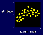
 The
figure shows data that lend themselves to fitting a polynomial. As you can see,
there is a so-called curvilinear trend in an outcome measure when it is
plotted against an independent variable. In the example the dependent variable
is some sort of attitude in athletes, but it could be performance or just about
anything. The independent variable is often some measure of time--here it's years
of competitive experience. Maybe the athletes start to go stale in this sport
after a certain time, and you'd like to be able to say so, quantitatively, with
confidence limits. Polynomial regression is the answer for these data and for
most curvilinear data that either show a maximum or a minimum in the curve, or
that could show a max or min if you extrapolated the curve beyond your data. Log
transformation is more likely to fit a curve that shows an ever-increasing
or ever-decreasing trend, although often it makes sense to fit a polynomial to
log-transformed data.
Often the different points come from the same subjects, especially when time
is the independent variable. You can still fit polynomials to such data, but
you have to use repeated-measures models. I deal
with repeated-measures polynomials
later, but the interpretation of the numbers describing the shape of the curve
is the same, and I deal with that here.
A Simple Polynomial
model: numeric <= numeric numeric2 numeric3...
example:
attitude <= experience experience2
Notice the subtle difference from the model
for multiple linear regression on the previous page.
Here the numbers 2, 3... represent powers of the same variable.
It might be easier to see if I write: Y <= X X2 X3... The
stats program fits the polynomial Y = a + bX + cX2 + dX3...
to the data. Polynomials are a special case of the more general non-linear
models. Check that page out again right now!
For data that are shaped like a parabola, you probably won't need more than
a quadratic model (Y <= X X2).
If the curve is trends up again at one end, you'll need a cubic model. Curves
with multiple kinks need even higher-order terms. It's rare to go past a quadratic,
though.
When you fit a model like Y <= X X2,
the stats program finds the best quadratic curve to fit the data. In other words,
it will find the best values for the coefficients (or parameters) a,
b and c in the equation Y = a + bX + cX2. The value of a represents the overall position of the
curve up and down the Y axis; for example, an increase of 1 unit in a shifts
the whole curve up the Y axis by 1 unit. The value of b represents the amount
of overall upward or downward linear (straight-line) trend in the values of
Y as you move along the X axis; in other words, if you draw a straight line
to fit all the points well, b is the slope of the line, which is the same thing
as the increase (or decrease, if b is negative) in Y for each 1-unit increase
in X. For the data in the figure, b would represent the change in attitude per
year of experience. The value of c represents the amount of curvature in the
data; in the present example, c would be negative, because the parabola is upside
down. I find it easier to interpret c visually if I transform the X values so
they range from -1 to +1. If I then fit a curve with this new independent variable,
the value of c that I get is about the amount that the values of Y sit above
(or fall below, if c is negative) a straight line at either end of the X range.
Remember that you can derive these coefficients or parameters as raw values,
as percents, and as normalized regression coefficients, just like the slope
in a simple linear regression. Make sure you interpret their magnitudes
and their confidence limits!
Caution! The linear term in a quadratic polynomial represents the overall
effect as you go from low to high values of the independent variable. The quadratic
term doesn't impact this overall effect--in fact, including the quadratic when
there is curvature in the trend will make the estimate of the linear term more
precise. But if you include a cubic term in the polynomial, the cubic
also contributes to the overall effect of going from low to high values of the
independent variable. This extra contribution of the cubic makes it impossible
to interpret the linear term as representing the difference between low and
high values of the independent variable. This problem is particularly important
when you are using polynomial contrasts in a
repeated-measures analysis, where the independent variable is time or trial
number. The easiest way to avoid the problem is to avoid including a cubic or
quintic in the polynomial. If you do include these higher order terms, and you
want an estimate of the difference between the effect of low and high values
of the independent variable (e.g., first test vs last test), you will have to
derive an estimate for the high minus the low values.
Don't forget that you can assess the contribution of each term of the polynomial
to the variance explained (R2) by the model. If your stats program doesn't give you
the R2 for each term, find the total sum of
squares and the sums of squares for each effect in the output, then calculate
the R2 for the quadratic term by dividing
its sum of squares by the total sum of squares, multiplied by 100 to convert
it to a percent. Phew! Interpret the R2 by
taking its square root and working out the confidence limits of the resulting
correlation, as described earlier.
A Polynomial With a Nominal Effect
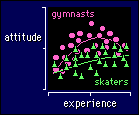
 The next figure shows an extension of
the above model to test for differences between two sports. Let's build up the
model term by term. We'll need sport as a main effect, to see how much overall
difference there is in the mean attitude for the two sports:
attitude <= sport
The main trend with experience is linear, and we want to know
about the differences in the slopes, so we need a full ANCOVA model:
attitude <= sport experience sport*experience
And finally, there is curvature for at least one sport, so we need
to fit a quadratic term overall, and a quadratic term that might
differ between the two sports. The way to do that is to include the
quadratic term as a main effect and as an interaction with sport. So
here's the full model:
attitude <= sport experience sport*experience experience2 sport*experience2
The p value for sport*experience2 tells you whether any difference in the
curvature for the two sports is statistically significant. Once again
you express this difference as a contribution to the overall
R2 for the model, as described for
the simpler example above.
Go to: Next · Previous · Contents · Search
· Home
webmaster=AT=newstats.org
Last updated 10 Dec 00
 The next figure shows an extension of
the above model to test for differences between two sports. Let's build up the
model term by term. We'll need sport as a main effect, to see how much overall
difference there is in the mean attitude for the two sports:
 The
figure shows data that lend themselves to fitting a polynomial. As you can see,
there is a so-called curvilinear trend in an outcome measure when it is
plotted against an independent variable. In the example the dependent variable
is some sort of attitude in athletes, but it could be performance or just about
anything. The independent variable is often some measure of time--here it's years
of competitive experience. Maybe the athletes start to go stale in this sport
after a certain time, and you'd like to be able to say so, quantitatively, with
confidence limits. Polynomial regression is the answer for these data and for
most curvilinear data that either show a maximum or a minimum in the curve, or
that could show a max or min if you extrapolated the curve beyond your data. Log
transformation is more likely to fit a curve that shows an ever-increasing
or ever-decreasing trend, although often it makes sense to fit a polynomial to
log-transformed data.